1. Get started with rbms - phenology
From counts to flight curve
Reto Schmucki (UKCEH)
28 November 2019
Source:vignettes/Get_Started_1.Rmd
Get_Started_1.RmdIn this tutorial, we show how to fit the flight curve function on
butterfly counts recorded on a weekly base. We use the R functions
implemented in the rbms package and the data bundle within
the same package. The data are genuine Butterfly Monitoring Scheme
counts with transect visit dates. The flight curve computation is based
on spline fitted on the counts collected across multiple sites and
standardised to sum to 1 (area under the curve is one).
1. load package and data included in the package
##  Welcome to rbms, version 1.1.3
##  This package has been tested, but is still in active development and feedbacks are welcome
## https://github.com/RetoSchmucki/rbms/issuesHere, the visit and count data are both packaged in data.table format but can also be provided as data.frame. The function converts them into data.table because this format is more efficient for handling large data sets. While the input format can vary, the header names need to be consistent, and some columns are essential for the functions to work.
Visit data represent the visit date at which each site was visited, and butterflies were monitored. If no butterfly was observed during a visit, the abundance for that specific visit would be set to zero [0]. This allows to subset positive non-zero counts from the count data set, which result in smaller objects to handle. The visit data may contain many columns, but only two are essential for the function.
- SITE_ID (can be numbers of characters and treated as a non-numeric factor)
- DATE (by default, the format is “%Y-%m-%d” (e.g., 2019-11-28]). If a different format needs to be specified, use the argument DateFormat)
##        SITE_ID       DATE
##          <int>     <char>
##     1:       1 2000-04-07
##     2:       1 2000-04-19
##     3:       1 2000-05-12
##     4:       1 2000-05-15
##     5:       1 2000-05-24
##    ---
## 12136:     193 2004-08-19
## 12137:     193 2004-08-31
## 12138:     193 2004-09-04
## 12139:     193 2004-09-15
## 12140:     193 2004-09-28
Count data must be provided in columns with specific headers; more column can be provided, but rbms only use the following four:
- SITE_ID
- DATE
- SPECIES
- COUNT
##       SITE_ID       DATE SPECIES   DAY MONTH  YEAR COUNT
##         <int>     <char>   <int> <int> <int> <int> <int>
##    1:       1 2000-04-07       2     7     4  2000     5
##    2:       1 2000-04-19       2    19     4  2000     3
##    3:       1 2000-05-12       2    12     5  2000     1
##    4:       1 2000-05-12       4    12     5  2000     2
##    5:       1 2000-05-15       4    15     5  2000     4
##   ---
## 5303:     193 2003-09-06       2     6     9  2003     1
## 5304:     193 2004-04-23       2    23     4  2004     2
## 5305:     193 2004-05-02       2     2     5  2004     1
## 5306:     193 2004-06-19       2    19     6  2004     2
## 5307:     193 2004-07-10       2    10     7  2004     1
2. organise the data to cover the time period and monitoring season of the BMS
With the visit and count data, we need to merge them into a new data.table object that covers the entire time-series of interest. This time-series is structured with the start and end date of the monitoring season and define on a weekly or a daily base (resolution of the flight curve). In a first step, we initialise the time-series with day-week-month-year information.
2.1. First, we initialise a time-series with day-week-month-year information.
ts_date <- rbms::ts_dwmy_table(InitYear = 2000, LastYear = 2003, WeekDay1 = 'monday')2.2. Ddd the monitoring season to the time-series
We add the monitoring season to the new time-series, providing the StartMonth and EndMonth arguments. The definition of the monitoring season can be refined with more arguments (StartDay, EndDay). We also define the resolution of the time-series (weekly or daily), where TimeUnit = ‘w’ will compute the flight curve based on weekly counts. In the alternative, ‘d’ is used for building a daily based flight curve. The ANCHOR argument adds zeros (0) before and after the monitoring season. This ensures that the flight curve starts and end at zero.
ts_season <- rbms::ts_monit_season(ts_date, StartMonth = 4, EndMonth = 9, StartDay = 1, EndDay = NULL, CompltSeason = TRUE, Anchor = TRUE, AnchorLength = 2, AnchorLag = 2, TimeUnit = 'w')NOTE: for species with overwintering adult and early counts, having an Anchor set to zero might sound wrong, and we are currently working on finding an alternative for these cases to represent the flight curve of those species better.
2.3. Add site visits to the time-series After the
monitoring season is defined for a specific time-period and monitoring
season, we use the ts_monit_site() function to expand and
inform the time-series with the site visits. For this, we use the visit
data and link it with the time series contained in ts_season object.
ts_season_visit <- rbms::ts_monit_site(m_visit, ts_season)## Warning in rbms::ts_monit_site(m_visit, ts_season): We have changed the order
## of the input arguments, with ts_seaon now in first place, before m_visit.2.4. Add observed count
The observed counts are then added to the time-series contained in
the data.table object, using the count and selecting the
species of interest with the argument sp. Here we use the
count recorded for species “2” (species names can also be a string of
characters).
ts_season_count <- rbms::ts_monit_count_site(ts_season_visit, m_count, sp = 2)The resulting data.table object contains zeros and
positive counts recorded along each BMS transects for species
2, over the entire time-series, but only within the focal
monitoring season. This time-series contains the week or days of the
counts. When the counts are missing because the site was not visited,
the count is informed as NA.
3. Compute the yearly flight curve for the data
With the object constructed above, we can compute the flight curve
for each year with sufficient data. The flight_curve
function assumes that the annual phenology shares the same shape across
sites.
The objective of this function is to extract this shape that we call the flight curve. Here, we want to impose some minimal threshold to control the quality of the data used to inform this model. This is done by setting the Minimum number of visits MinNbrVisit, the minimum number of occurrences MinOccur and the number of sites MinNbrSite to use to fit the model.
These values can influence the model, and its sensitivity will depend on the species and the data set. Still, as a minimum requirement, MinOccur should be set >= 2, the MinNbrVisit > MinOccur and MinNbrSite >= 5. These thresholds affect the data that inform your model and the resulting flight curve. When higher values are chosen, fewer sites will be available and if insufficient, the thresholds need to be revised.
ts_flight_curve <- rbms::flight_curve(ts_season_count, NbrSample = 300, MinVisit = 5, MinOccur = 3, MinNbrSite = 5, MaxTrial = 4, GamFamily = 'nb', SpeedGam = FALSE, CompltSeason = TRUE, SelectYear = NULL, TimeUnit = 'w')## Fitting the flight curve spline for species 2 and year 2000 with 76 sites, using gam() : 2024-07-26 13:17:30.156215 -> trial 1## Fitting the flight curve spline for species 2 and year 2001 with 76 sites, using gam() : 2024-07-26 13:17:31.287699 -> trial 1## Fitting the flight curve spline for species 2 and year 2002 with 87 sites, using gam() : 2024-07-26 13:17:31.858448 -> trial 1## Fitting the flight curve spline for species 2 and year 2003 with 103 sites, using gam() : 2024-07-26 13:17:32.590657 -> trial 1NOTE: for the
flight_curvefunction, you will also have to define some parameters for the distribution for the GAM model as well as the maximum number of times to try to fit the model and the number of samples to use. The later will take a random sample from the data set if it contains more site than the number specified.
From the flight_curve() function, we can retrieve a list of 3 objects:
- pheno that contain the standardised phenology curve derived by fitting a GAM model, with a cubic spline to the count data;
- model that contains the result of the fitted GAM model;
- data the data used to fit the GAM model.
We can now extract the pheno object, a data.frame that contains the shape of the annual flight curves, standardised to sum to 1. The flight-curves contained in the pheno object can be visualised with the following line of codes.
Note for purpose of demonstration, let’s imagine that we could not fit a flight curve for year 2002 and the flight curve returned “NA” for that year 2002. Our code needs to be aware of the missing year.
## Extract phenology part
pheno <- ts_flight_curve$pheno

## add the line of the first year
yr <- unique(pheno[order(M_YEAR),][!is.na(NM), as.numeric(as.character(M_YEAR))])

if("trimWEEKNO" %in% names(pheno)){
  plot(unique(pheno[M_YEAR == yr[1], .(trimWEEKNO, NM)]), type = 'l', ylim = c(0, max(pheno[!is.na(NM), ][, NM])), xlab = 'Monitoring Week', ylab = 'Relative Abundance')
} else {
  plot(unique(pheno[M_YEAR == yr[1], .(trimDAYNO, NM)]), type = 'l', ylim = c(0, max(pheno[!is.na(NM), ][, NM])), xlab = 'Monitoring Day', ylab = 'Relative Abundance')

}
## add individual curves for additional years
if(length(yr) > 1) {
i <- 2
  for(y in yr[-1]){
    if("trimWEEKNO" %in% names(pheno)){
      points(unique(pheno[M_YEAR == y , .(trimWEEKNO, NM)]), type = 'l', col = i)
    } else {
      points(unique(pheno[M_YEAR == y, .(trimDAYNO, NM)]), type = 'l', col = i)
    }
    i <- i + 1
  }
}

## add legend
legend('topright', legend = c(yr), col = c(seq_along(c(yr))), lty = 1, bty = 'n')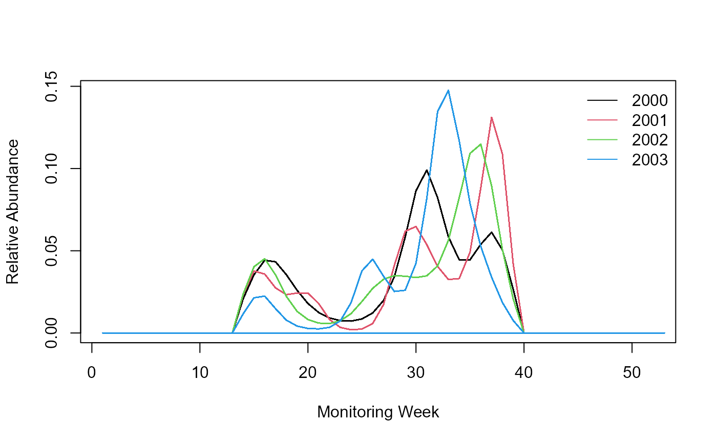
Flight curve.
The code above produces a flight curve for each of the four years. Now, let’s imagine that the model could not fit a flight curve for year 2002 and the flight curve returned “NA” for that year 2002. Our code needs to be aware of the missing year and skip that year.
## Extract phenology part
pheno <- pheno[M_YEAR == 2002, NM := NA]

## add the line of the first year
yr <- unique(pheno[order(M_YEAR),][!is.na(NM), as.numeric(as.character(M_YEAR))])

if(length(yr) > 0){ # need at least one year without "NA" for the flight curve

if("trimWEEKNO" %in% names(pheno)){
  plot(unique(pheno[M_YEAR == yr[1], .(trimWEEKNO, NM)]), type = 'l', ylim = c(0, max(pheno[!is.na(NM), ][, NM])), xlab = 'Monitoring Week', ylab = 'Relative Abundance')
} else {
  plot(unique(pheno[M_YEAR == yr[1], .(trimDAYNO, NM)]), type = 'l', ylim = c(0, max(pheno[!is.na(NM), ][, NM])), xlab = 'Monitoring Day', ylab = 'Relative Abundance')

}
## add individual curves for additional years
if(length(yr) > 1) {
i <- 2
  for(y in yr[-1]){
    if("trimWEEKNO" %in% names(pheno)){
      points(unique(pheno[M_YEAR == y , .(trimWEEKNO, NM)]), type = 'l', col = i)
    } else {
      points(unique(pheno[M_YEAR == y, .(trimDAYNO, NM)]), type = 'l', col = i)
    }
    i <- i + 1
  }
}
}

## add legend
legend('topright', legend = c(yr), col = c(seq_along(c(yr))), lty = 1, bty = 'n')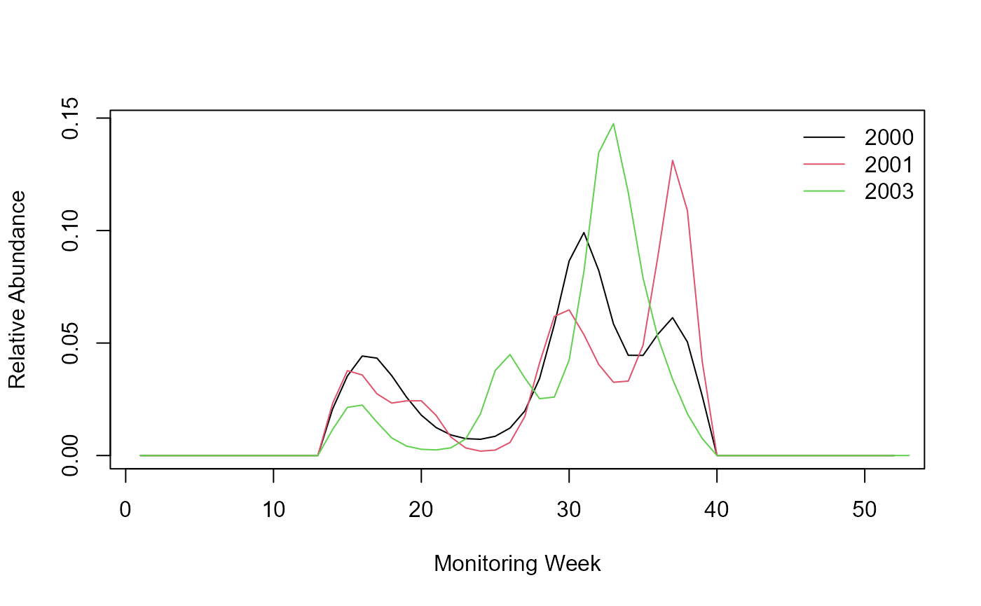
Flight curve without (2002=NA).