2. Get started with rbms - collate index
Inputting missing counts
Reto Schmucki (UKCEH)
28 November 2019
Source:vignettes/Get_Started_2.Rmd
Get_Started_2.RmdFrom the flight curve and the observed counts, we can derive expected values for weeks or days where a site has not been monitored. Together, observed and imputed counts are used to compute abundance indices across sites. Site indices are then used to calculate annual collated indices.
see 1. Get started with
rbmsto compute the flight curve object used below (Step 1, 2 and 3)
##  Welcome to rbms, version 1.1.3
##  This package has been tested, but is still in active development and feedbacks are welcome
##  https://github.com/RetoSchmucki/rbms/issues
data(m_visit)
data(m_count)
ts_date <- rbms::ts_dwmy_table(InitYear = 2000, LastYear = 2003, WeekDay1 = 'monday')
ts_season <- rbms::ts_monit_season(ts_date, StartMonth = 4, EndMonth = 9, StartDay = 1, EndDay = NULL, CompltSeason = TRUE, Anchor = TRUE, AnchorLength = 2, AnchorLag = 2, TimeUnit = 'w')
ts_season_visit <- rbms::ts_monit_site(m_visit, ts_season)
## Warning in rbms::ts_monit_site(m_visit, ts_season): We have changed the order
## of the input arguments, with ts_seaon now in first place, before m_visit.
ts_season_count <- rbms::ts_monit_count_site(ts_season_visit, m_count, sp = 2)
ts_flight_curve <- rbms::flight_curve(ts_season_count, NbrSample = 300, MinVisit = 5, MinOccur = 3, MinNbrSite = 5, MaxTrial = 4, GamFamily = 'nb', SpeedGam = FALSE, CompltSeason = TRUE, SelectYear = NULL, TimeUnit = 'w')
## Fitting the flight curve spline for species 2 and year 2000 with 76 sites, using gam() : 2024-07-26 13:17:46.161633 -> trial 1## Fitting the flight curve spline for species 2 and year 2001 with 76 sites, using gam() : 2024-07-26 13:17:48.630974 -> trial 1## Fitting the flight curve spline for species 2 and year 2002 with 87 sites, using gam() : 2024-07-26 13:17:50.681385 -> trial 1## Fitting the flight curve spline for species 2 and year 2003 with 103 sites, using gam() : 2024-07-26 13:17:53.169702 -> trial 14. Impute predicted counts for missing monitoring dates
The impute_count() function uses the count data
generated from the ts_season_count() function and the
flight curves (ts_flight_curve$pheno) obtained from the
flight_curve() function. The impute_count()
function looks for the phenology available (using the nearest year) to
estimate and input missing values; the extend of the search for nearest
phenology can be limited by setting the YearLimit parameter. By default,
this is not restricted and will look over all years available. Like
other rbms functions, the imputation can be made on a weekly or daily
basis (‘w’ or ‘d’).
## extract phenology data from the ts_fligh_curve list
pheno <- ts_flight_curve$pheno
## note: extraction of the pheno part is not necessary any more, as this is now done internally if not yet extract. Nevertheless the process still work and remains backward compatible.
## ts_flight_curve = ts_flight_curve would also work

impt_counts <- rbms::impute_count(ts_season_count=ts_season_count, ts_flight_curve=pheno, YearLimit= NULL, TimeUnit='w')
The impute_count() function produces a data.table that
contains the original COUNT values, a series of IMPUTED_COUNT over
monitoring season, TOTAL_COUNT per site and year, TOTAL_NM (e.g. the
proportion of the flight curve covered by the visits) and SINDEX. The
SINDEX is the site index that corresponds to the sum of both observed
and imputed counts over the sampling season. If the flight curve of a
specific year is missing, the impute_count() function uses
the nearest phenology found. If none is available within the limit of
years set by the YearLimit parameter, the function will return no SINDEX
for that specific year.
impt_counts_1year <- rbms::impute_count(ts_season_count=ts_season_count, ts_flight_curve=pheno[M_YEAR != 2001, ], YearLimit= 1, TimeUnit='w')## Warning in FUN(X[[i]], ...): We used the flight curve of 2000 to compute
## abundance indices for year 2001
impt_counts_0year <- rbms::impute_count(ts_season_count=ts_season_count, ts_flight_curve=pheno[M_YEAR != 2001, ], YearLimit= 0, TimeUnit='w')## No reliable flight curve available within a 0 year horizon of 20015. Site and collated indices
From the imputed count, the site index can be calculated for each site or with a filter that will only keep sites that have been monitored at least a certain proportion of the flight curve. In this example, we set the threshold to 10%, using the MinFC parameter.
sindex <- rbms::site_index(butterfly_count = impt_counts, MinFC = 0.10)With the site indices, annual collated indices can be estimated by fitting a Generalised Linear Model (GLM), where sites and years are modelled as factors. Here we also use the proportion of the flight curve sampled by the observation as a weight for the GLM. Finally, we remove all sites where the species was not observed, setting the parameter rm_zero = TRUE will facilitates model fit.
co_index <- collated_index(data = sindex, s_sp = 2, sindex_value = "SINDEX", glm_weights = TRUE, rm_zero = TRUE)The collated index computed by the collated_index()
function can be interpreted as the mean total butterfly count expected
on a BMS transect in a given year.
## $col_index
## Key: <M_YEAR>
##    BOOTi M_YEAR NSITE NSITE_B NSITE_OBS COL_INDEX
##    <num>  <num> <int>   <int>     <int>     <num>
## 1:     0   2000   124     124       107  18.22935
## 2:     0   2001   108     108       100  30.15065
## 3:     0   2002   114     114       107  30.66658
## 4:     0   2003   122     122       113  59.78319
##
## $site_id
##   [1] "1"   "14"  "157" "158" "159" "160" "161" "162" "163" "164" "165" "166"
##  [13] "15"  "167" "168" "169" "170" "171" "172" "173" "174" "175" "176" "16"
##  [25] "177" "178" "179" "185" "193" "51"  "82"  "31"  "41"  "154" "19"  "180"
##  [37] "181" "182" "187" "183" "184" "186" "21"  "23"  "24"  "25"  "26"  "27"
##  [49] "2"   "28"  "29"  "30"  "32"  "34"  "36"  "37"  "39"  "42"  "43"  "3"
##  [61] "45"  "47"  "48"  "54"  "60"  "61"  "62"  "64"  "65"  "69"  "4"   "71"
##  [73] "72"  "76"  "83"  "84"  "85"  "86"  "89"  "91"  "92"  "6"   "93"  "95"
##  [85] "96"  "97"  "99"  "100" "101" "102" "104" "106" "8"   "107" "111" "112"
##  [97] "113" "115" "116" "117" "118" "119" "120" "9"   "122" "123" "124" "126"
## [109] "127" "128" "129" "130" "132" "133" "10"  "134" "135" "136" "137" "139"
## [121] "140" "141" "142" "143" "144" "12"  "145" "146" "147" "148" "149" "150"
## [133] "151" "153" "155" "156"
The index can be transformed to a log(10) scale
co_index <- co_index$col_index
co_index_b <- co_index[COL_INDEX > 0.0001 & COL_INDEX < 100000, ]
co_index_logInd <- co_index_b[BOOTi == 0, .(M_YEAR, COL_INDEX)][, log(COL_INDEX)/log(10), by = M_YEAR][, mean_logInd := mean(V1)]

## merge the mean log index with the full bootstrap dataset
data.table::setnames(co_index_logInd, "V1", "logInd"); setkey(co_index_logInd, M_YEAR); setkey(co_index_b, M_YEAR)
co_index_b <- merge(co_index_b, co_index_logInd, all.x = TRUE)
The log scaled indices can then be plotted with the following code;
here we represent the data with time-series average being centred to two
(i.e. log10(100)).
col_pal <- c("cyan4", "orange", "orangered2")

## compute the metric used for the graph of the Collated Log-Index centred around 2 (observed, bootstrap sample, credible confidence interval, linear trend)
b1 <- data.table(M_YEAR = co_index_b$M_YEAR, LCI = 2 + co_index_b$logInd - co_index_b$mean_logInd)
b2 <- data.table(M_YEAR = co_index_b[BOOTi == 0, M_YEAR], LCI= 2 + co_index_b[BOOTi == 0, logInd] - co_index_b[BOOTi == 0, mean_logInd])

lm_mod <- try(lm(LCI ~ M_YEAR, data = b2), silent=TRUE)

plot(b1, col = adjustcolor( "cyan4", alpha.f = 0.2),
      xlab = "year", ylab = expression('log '['(10)']*' Collated Index'),
      xaxt="n", type = 'n')

axis(1, at = b2$M_YEAR)

points(b2[!is.na(LCI),], type = 'l', lty=2, col="grey70")
points(b2, type = 'l', lwd=1.3, col = col_pal[1])
points(b2[!is.na(LCI),], col= col_pal[1], pch=19)
abline(h=2, lty=2)

if (class(lm_mod)[1] != "try-error"){
    points(b2$M_YEAR, as.numeric(predict(lm_mod, newdata = b2, type = "response")),
    type = 'l', col='maroon4', lwd = 1.5, lty = 1)
  }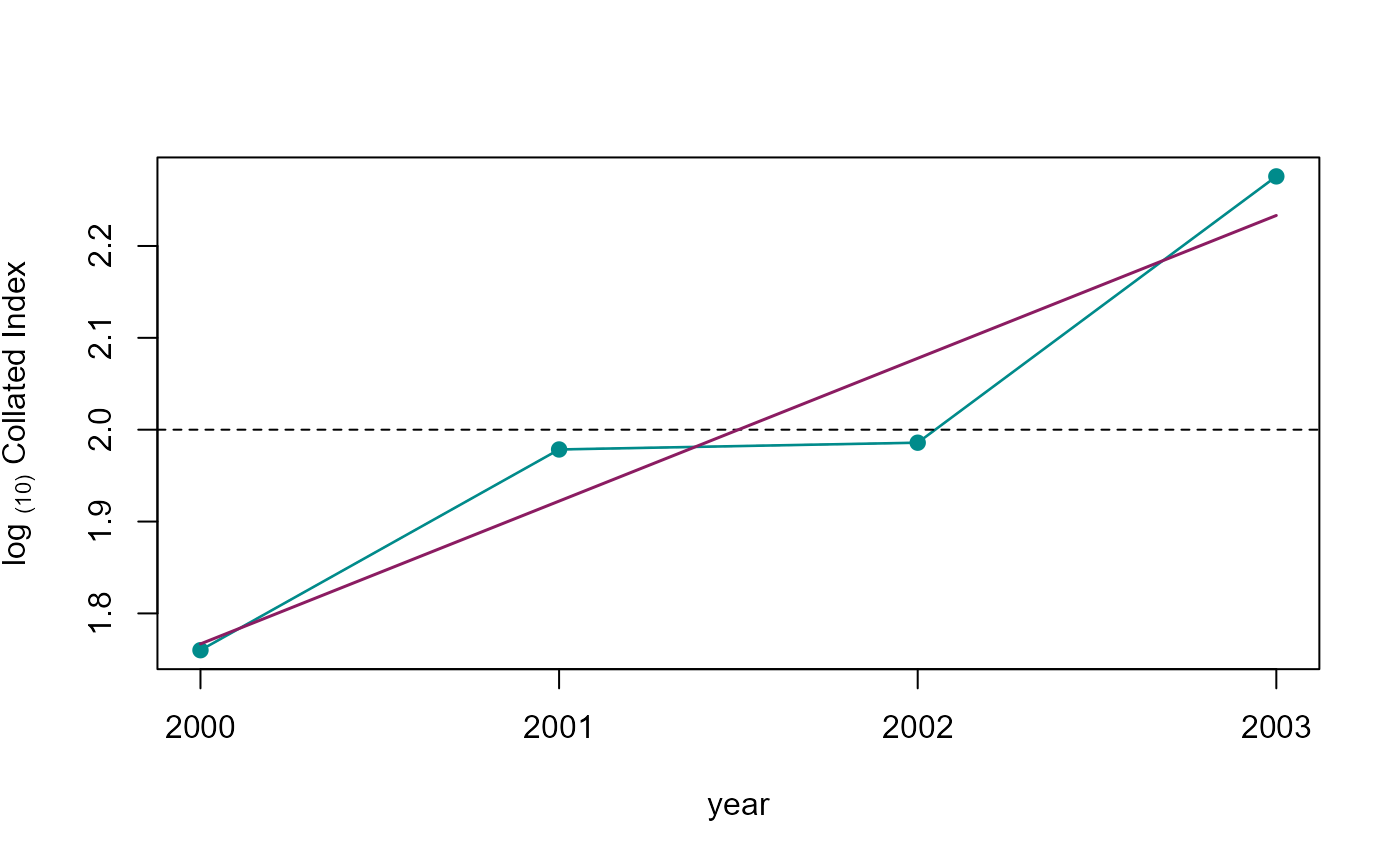
Collated index.
6. Bootstrap confidence interval
The confidence interval around the collated indices can be computed from a bootstrap sample, where n site indices are randomly resampled (with replacement) k time to produce a distribution of the annual collated indices. From this distribution, we can derive the confidence intervals around the collated indices. We first define k bootstrap sample using the function boot_sample(). Here we set k to 200 samples, but for a reliable confidence interval, k should be at least 1000. For reproducibility, we use set.seed() to generate a repeatable random sample
set.seed(218795)
bootsample <- rbms::boot_sample(sindex, boot_n = 200)
Using the collated_index() function in a loop, with
bootstrap samples informing the argument boot_ind, we can
now compute k collated indies over the entire time-series.
co_index <- list()

## for progression bar, uncomment the following
## pb <- txtProgressBar(min = 0, max = dim(bootsample$boot_ind)[1], initial = 0, char = "*",  style = 3)

for(i in c(0,seq_len(dim(bootsample$boot_ind)[1]))){

 co_index[[i+1]] <- rbms::collated_index(data = sindex, s_sp = 2, sindex_value = "SINDEX", bootID=i, boot_ind= bootsample, glm_weights=TRUE, rm_zero=TRUE)

## for progression bar, uncomment the following
## setTxtProgressBar(pb, i)

}

## collate and append all the result in a data.table object
co_index <- rbindlist(lapply(co_index, FUN = "[[","col_index"))
Annual log indices, as well as their average, are then computed from the original sample. Similarly, we compute annual log indices for each bootstrap sample.
co_index_b <- co_index[COL_INDEX > 0.0001 & COL_INDEX < 100000, ]
co_index_logInd <- co_index_b[BOOTi == 0, .(M_YEAR, COL_INDEX)][, log(COL_INDEX)/log(10), by = M_YEAR][, mean_logInd := mean(V1)]

## merge the mean log index with the full bootstrap dataset
data.table::setnames(co_index_logInd, "V1", "logInd"); setkey(co_index_logInd, M_YEAR); setkey(co_index_b, M_YEAR)
co_index_b <- merge(co_index_b, co_index_logInd, all.x = TRUE)

data.table::setkey(co_index_b, BOOTi, M_YEAR)
co_index_b[ , boot_logInd := log(COL_INDEX)/log(10)]
From the bootstrap samples, we can derive a 95% Confidence Interval, using the corresponding percentiles (i.e., 0.025 and 0.975).
b1 <- data.table(M_YEAR = co_index_b$M_YEAR, LCI = 2 + co_index_b$boot_logInd - co_index_b$mean_logInd)
b2 <- data.table(M_YEAR = co_index_b[BOOTi == 0, M_YEAR], LCI= 2 + co_index_b[BOOTi == 0, logInd] - co_index_b[BOOTi == 0, mean_logInd])
b5 <- b1[co_index_b$BOOTi != 0, quantile(LCI, 0.025, na.rm = TRUE), by = M_YEAR]
b6 <- b1[co_index_b$BOOTi != 0, quantile(LCI, 0.975, na.rm = TRUE), by = M_YEAR]
lm_mod <- try(lm(LCI ~ M_YEAR, data = b2), silent=TRUE)

## define graph axis limits and color scheme
yl <- c(floor(min(b5$V1, na.rm=TRUE)), ceiling(max(b6$V1, na.rm=TRUE)))

col_pal <- c("cyan4", "orange", "orangered2")

## draw the plot for the selected species
plot(b1, ylim = yl, col = adjustcolor( "cyan4", alpha.f = 0.2),
      xlab = "year", ylab = expression('log '['(10)']*' Collated Index'),
      xaxt="n", type = 'n')

axis(1, at = b2$M_YEAR)

segments(x0 = as.numeric(unlist(b5[,1])), y0 = as.numeric(unlist(b5[,2])),
         x1 = as.numeric(unlist(b6[,1])), y1 = as.numeric(unlist(b6[,2])),
         col = col_pal[2], lwd = 2)
points(b2[!is.na(LCI),], type = 'l', lty=2, col="grey70")
points(b2, type = 'l', lwd=1.3, col = col_pal[1])
points(b2[!is.na(LCI),], col= col_pal[1], pch=19)
abline(h=2, lty=2)

if (class(lm_mod)[1] != "try-error"){
    points(b2$M_YEAR, as.numeric(predict(lm_mod, newdata = b2, type = "response")),
    type = 'l', col='maroon4', lwd = 1.5, lty = 1)
  }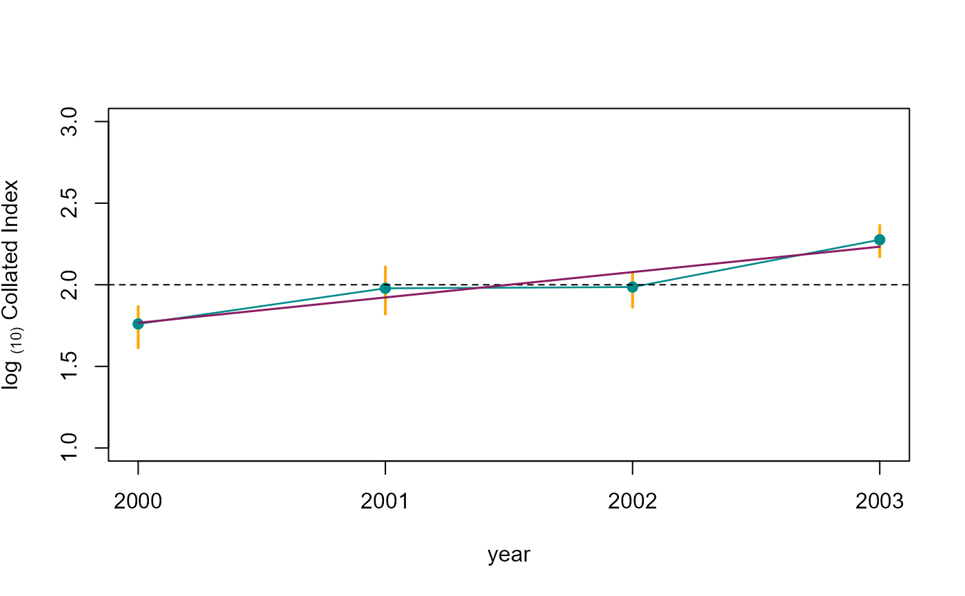
Collated index with 95% CI.