Bivoltine species

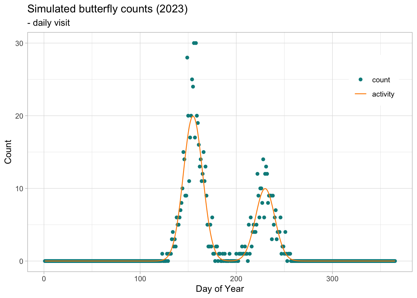
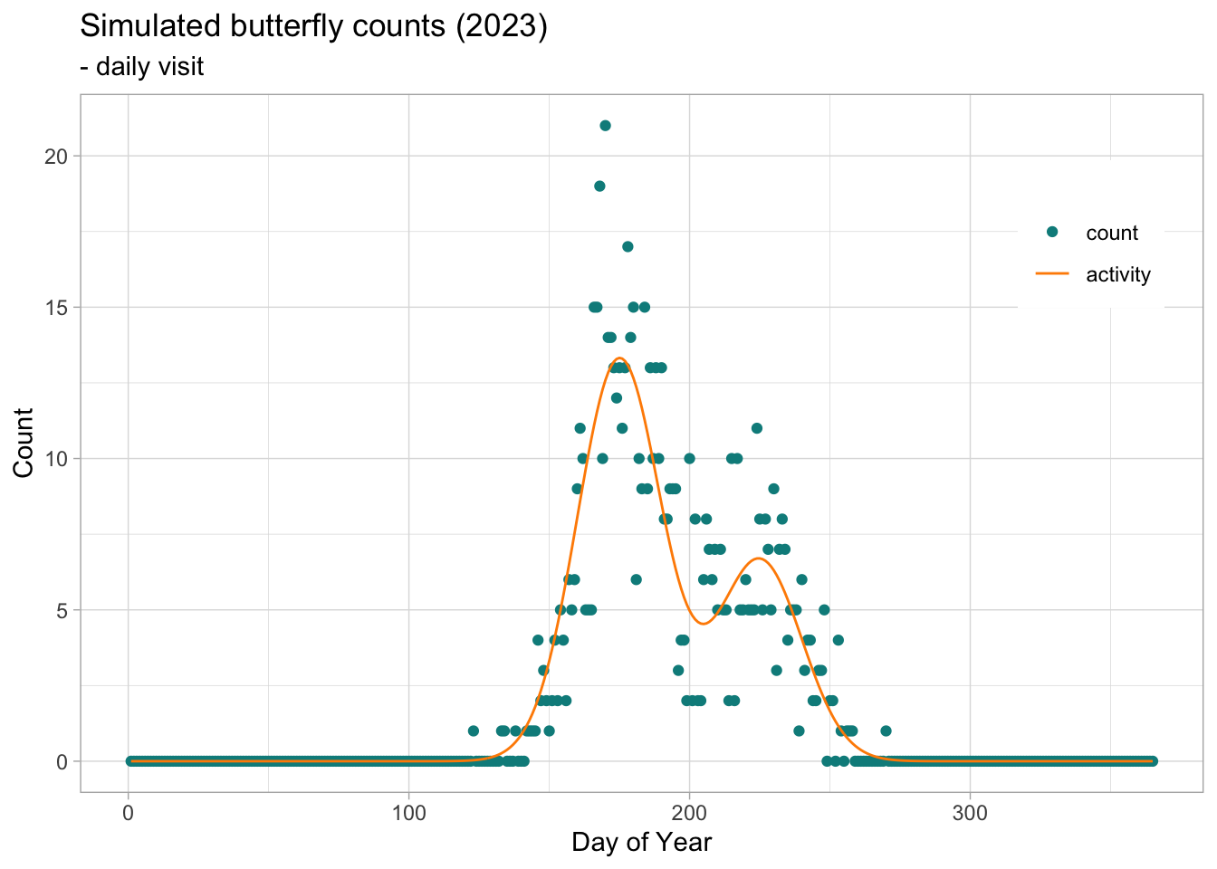
Some butterfly species produce more than one generation per year. This mean that the populations will produce successive generations within the monitoring season. This phenomenon will be reflected in the adult count, resulting in bimodal distributions when the two generations are sufficently spaced in time and that the overlap of the flight curve of the different cohort is not to large.

We can simulate bivoltine counts by simply overlapping two generation simulated independently, each with their specific parameters.

Code

set.seed(13276)

if(!require("rbms")) devtools::install_github("RetoSchmucki/rbms")
if(!require("butterflyGamSims")) devtools::install_github("cbedwards/butterflyGamSims")
if(!require("mixR")) devtools::install_github("RetoSchmucki/mixR") # small fix in plot function, not yet implemented in original and CRAN version

library(rbms)
library(mixR)
library(butterflyGamSims)
library(data.table)
library(ggplot2)

flc_col <- '#ff8c00'
cnt_col <- '#008b8b'
missing_col <- '#8b0000'
GAM_col <- '#483d8b'

## local functions
sim2bms <- function(data, yearKeep = NULL, weeklySample = FALSE, weekdayKeep = NULL, monitoringSeason = NULL){
                  
                  btfl_ts <- data.table::data.table(data)[, site_id := paste0("site_",sim.id)]
                  if(!is.null(yearKeep)){
                        btfl_ts <- btfl_ts[years %in% yearKeep, ]
                  }
                  btfl_ts[ , date := as.Date(doy, origin = paste0(years, "-01-01"))-1]
                  btfl_ts[ , week := isoweek(date)]
                  btfl_ts[month(date) != 1 | week < 50, weekday := rowid(week), by = .(site_id, years)]
                  if(isTRUE(weeklySample)){
                        if(!is.null(weekdayKeep)){
                              btfl_ts <- btfl_ts[weekday %in% weekdayKeep, ]
                        }
                        btfl_ts <- btfl_ts[btfl_ts[,.I[sample(.N, 1)], by = .(week, site_id, years)][["V1"]],]
                  }
                  if(!is.null(monitoringSeason)){
                  btfl_ts <- btfl_ts[month(date) %in% monitoringSeason, ]
                  }
            return(btfl_ts)
            }

missing_prob <- function(data, mu=NULL, alpha = 5, theta = 0.3){
                              x_ <- seq_len(nrow(data))
                              mu_ <- ifelse(is.null(mu), length(x_) / 2, mu)
                              std_ <- sqrt(mu_ / theta)
                              y_ <- abs((alpha * exp((-(x_ - mu_)^2) / std_^2)) - alpha) + alpha
                              yn_ <- y_ / (sum(y_))
                        return(yn_)
                  }

sample_missing <- function(data, propMissing = 0.25){
            
            missing.prob <- data.table::data.table()
            for(i in data[, unique(years)]){
                  for(j in data[, unique(site_id)]){
                  missing.prob <- rbind(missing.prob, missing_prob(data[years == i & site_id == j, ]))
                  }
            }
            
            missing.week <- data[sample(seq_len(.N), round(propMissing * .N), prob = unlist(missing.prob)), ]  
      
      return(missing.week)
}

Code

size1 <- 500
peak1 <- 155
sd1 <- 10
size2 <- 250
peak2 <- 230
sd2 <- 10
y <- c(2023)

btfl_data1 <- timeseries_sim(nsims=1,
               year = y,
               doy.samples = seq(from=1, to=365, by=1),
               abund.type = "exp",
               activity.type = "gauss",
               sample.type = "pois",
               sim.parms = list(growth.rate = 0,
                                init.size = size1, 
                                act.mean = peak1,
                                act.sd = sd1)
               )

btfl_data2 <- timeseries_sim(nsims=1,
               year = y,
               doy.samples = seq(from=1, to=365, by=1),
               abund.type = "exp",
               activity.type = "gauss",
               sample.type = "pois",
               sim.parms = list(growth.rate = 0,
                                init.size = size2, 
                                act.mean = peak2,
                                act.sd = sd2)
               )

btfl_data_b2 <- rbind(btfl_data1$timeseries[,c("years", "doy", "count", "act", "sim.id")], 
                      btfl_data2$timeseries[,c("years", "doy", "count", "act", "sim.id")])
btfl_data_b2 <- unique(data.table(btfl_data_b2)[, ":="(count=sum(count), act=sum(act)), by = .(years, doy)])
btfl_data_b2[, abund.true:= sum(c(size1, size2))]

btfl_ts <- sim2bms(data = btfl_data_b2, yearKeep = y)

btfl_fig1 <- ggplot() +
                geom_point(data=btfl_ts, aes(x=doy, y=count, colour = "count")) + 
                geom_line(data = btfl_ts,
                aes(x = doy, y = act, colour = "activity")) +
                xlim(1,365) + ylim(0, max(btfl_ts$count, btfl_ts$act)) + 
                scale_colour_manual("", 
                      breaks = c("count", "activity"),
                      values = c(cnt_col, flc_col)) +
                theme_light() + 
                theme(legend.position = "inside", legend.position.inside = c(0.9, 0.8)) +
                labs(title = paste0("Simulated butterfly counts (", y,")"),
                     subtitle = "- daily visit",
                     x = "Day of Year",
                     y = "Count")
btfl_fig1

Code

## ===========================
## degradation1: weekly count
## ===========================

btfl_week_smpl <- sim2bms(data = btfl_data_b2, yearKeep = y, 
                  weeklySample = TRUE,
                  weekdayKeep = c(2:5),
                  monitoringSeason = c(4:9))

btfl_fig2 <- ggplot() +
                geom_point(data=btfl_week_smpl, aes(x=doy, y=count, colour = "count")) + 
                geom_line(data = btfl_ts,
                aes(x = doy, y = act, colour = "activity")) +
                xlim(1,365) + ylim(0, max(btfl_ts$count, btfl_ts$act)) + 
                scale_colour_manual("", 
                      breaks = c("count", "activity"),
                      values = c(cnt_col, flc_col)) +
                theme_light() + 
                theme(legend.position = "inside", legend.position.inside = c(0.9, 0.8)) +
                labs(title = paste0("Simulated butterfly counts (", y,")"),
                     subtitle = "- weekly visit (random resampled)",
                     x = "Day of Year",
                     y = "Count")

btfl_fig2

Code

## ==============================
## degradation: add missing week
## ==============================

btfl_week_missing <- sample_missing(data = btfl_week_smpl, propMissing = 0.25)

btfl_fig3 <- ggplot() +
                geom_point(data=btfl_week_smpl, aes(x=doy, y=count, colour = "count")) + 
                geom_point(data=btfl_week_missing, aes(x=doy, y=count, colour = "missing"), 
                            shape=4, size=2, stroke=2) + 
                geom_line(data = btfl_ts,
                aes(x = doy, y = act, colour = "activity")) +
                xlim(1,365) + ylim(0, max(btfl_ts$count, btfl_ts$act)) + 
                scale_colour_manual("", 
                      breaks = c("count", "activity", "missing"),
                      values = c(cnt_col, flc_col, missing_col)) +
                theme_light() + 
                theme(legend.position = "inside", legend.position.inside = c(0.9, 0.8)) +
                labs(title = paste0("Simulated butterfly counts (", y,")"),
                     subtitle = "- weekly visit (random resampled)",
                     x = "Day of Year",
                     y = "Count")

btfl_fig3

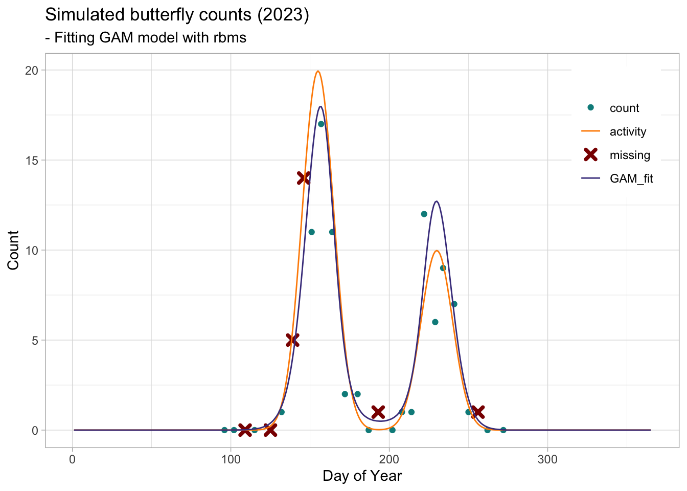
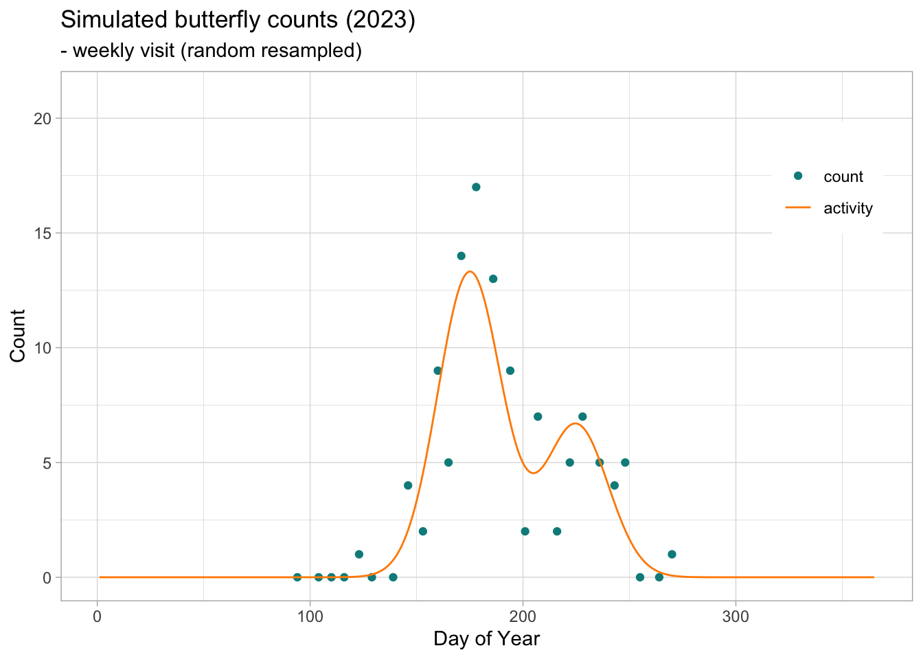
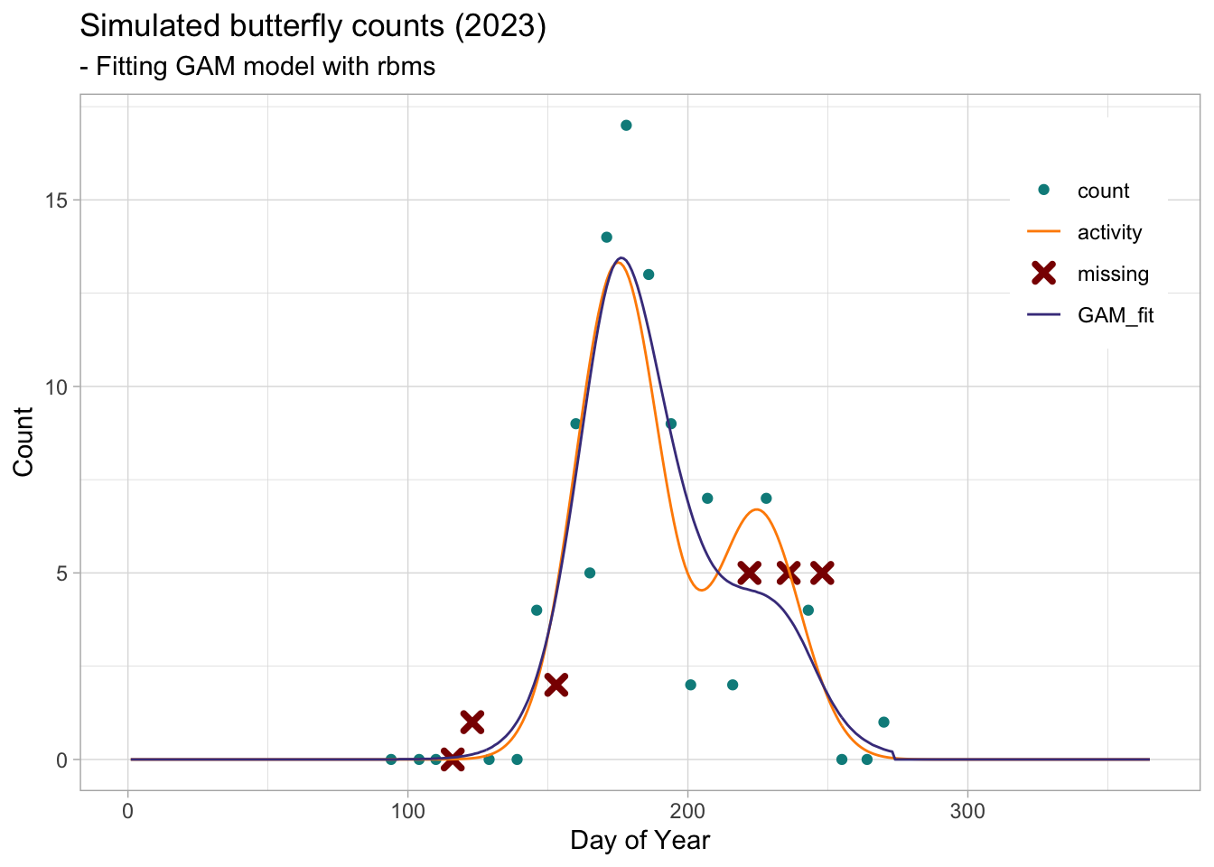
From the weekly counts recorded (simulated) for the bivoltine species, we can use the rbms package to fit a Generalized Additive Model (GAM) to retrieve the overall shape of the annual flith curve. Althouhg we only use one site here, this can be extended and more powerfull if we had more than one site monitored within the region.

Code

visit_sim <- btfl_week_smpl[!date %in% btfl_week_missing$date, .(site_id, date, count)]
count_sim <- visit_sim[count>=1,][, species := "sp1"]

names(visit_sim) <- toupper(names(visit_sim))
names(count_sim) <- toupper(names(count_sim))

ts_date <- rbms::ts_dwmy_table(InitYear = 2023, LastYear = 2023, WeekDay1 = 'monday')

ts_season <- rbms::ts_monit_season(ts_date,
                       StartMonth = 4,
                       EndMonth = 9, 
                       StartDay = 1,
                       EndDay = NULL,
                       CompltSeason = TRUE,
                       Anchor = TRUE,
                       AnchorLength = 2,
                       AnchorLag = 2,
                       TimeUnit = 'd')

ts_season_visit <- rbms::ts_monit_site(ts_season, visit_sim)

ts_season_count <- rbms::ts_monit_count_site(ts_season_visit, count_sim, sp = "sp1")

### Fitting a GAM to Butterfly Counts

ts_flight_curve <- rbms::flight_curve(ts_season_count, 
                       NbrSample = 300,
                       MinVisit = 5,
                       MinOccur = 3,
                       MinNbrSite = 1,
                       MaxTrial = 4,
                       GamFamily = 'nb',
                       SpeedGam = FALSE,
                       CompltSeason = TRUE,
                       SelectYear = NULL,
                       TimeUnit = 'd')


## plot-fitted-flight-curve

pheno <- ts_flight_curve$pheno

btfl_fig4 <- ggplot() +
                geom_point(data=ts_season_count[ANCHOR == 0 & !is.na(COUNT), ], aes(x=DAY_SINCE, y=COUNT, colour = "count")) +
                geom_point(data=btfl_week_missing, aes(x=doy, y=count, colour = "missing"), 
                            shape=4, size=2, stroke=2) + 
                geom_line(data = btfl_ts, aes(x = doy, y = act, colour = "activity")) +
                geom_line(data = pheno,
                    aes(x = trimDAYNO, y = btfl_ts[, unique(abund.true)]*NM, colour = "GAM_fit")) +
                xlim(1,365) + ylim(0, max(btfl_ts$act, 
                                          pheno$NM*btfl_ts[,unique(abund.true)], 
                                          btfl_week_missing$count, 
                                          ts_season_count[!is.na(COUNT), COUNT] )) + 
                scale_colour_manual("", 
                      breaks = c("count", "activity", "missing", "GAM_fit"),
                      values = c(cnt_col, flc_col, missing_col, GAM_col)) +
                theme_light() + 
                theme(legend.position = "inside", legend.position.inside = c(0.9, 0.8)) +
                labs(title = paste0("Simulated butterfly counts (", y,")"),
                     subtitle = "- Fitting GAM model with rbms",
                     x = "Day of Year",
                     y = "Count")
btfl_fig4

Retrieve Generation Parameters

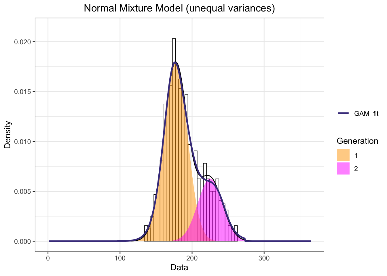
The GAM fitted very well the cummulative fligth curve (e.i., two generations activity curves). While the GAM returns the overall shape resulting from all observation the model does not distinguish the different generations. We can however fit a mixture model with k components (generations) to estimate and retrieve the parameters of the different generations. Here we will simply try to fit two generation with parameter of a Gaussian distribution (mean and standard deviation). The R package mixR provides an efficient algorithm (C++) to fit and assess the goodness of fit of such model(Yu 2022) .

Code

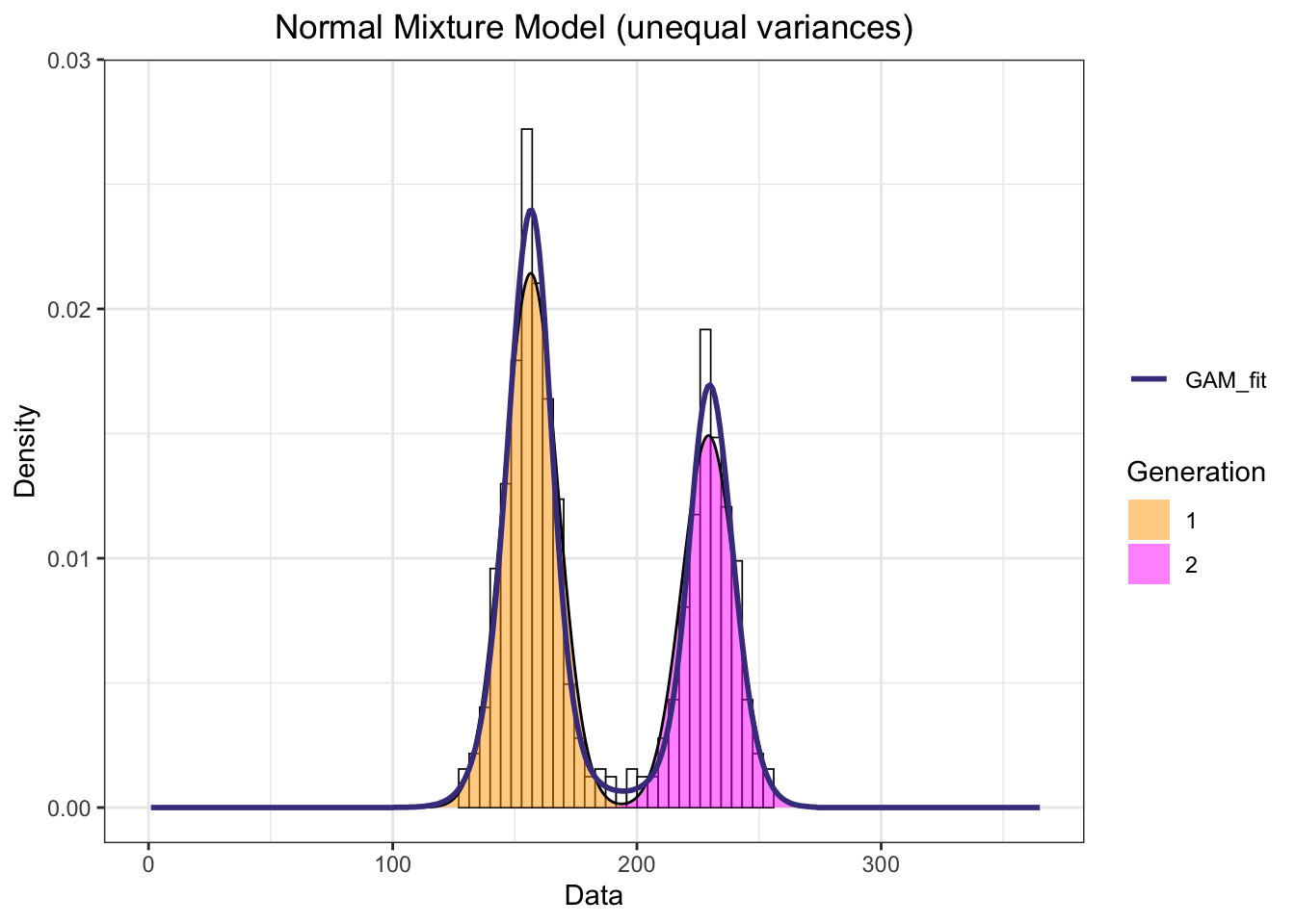
set.seed(102)
btnbr <- pheno$NM*btfl_ts[,unique(abund.true)]
x1 <- rep(1:365, round(btnbr))

# fit a Normal mixture model (unequal variances)
mod1 = mixfit(x1, ncomp = 2)
gen_plot1 <- plot(mod1, title = 'Normal Mixture Model (unequal variances)')

gen_plot1 +
      xlim(0, 365) + 
      scale_fill_manual("Generation", values=c("orange","magenta")) +
      geom_line(data = pheno, aes(x = trimDAYNO, y = NM, colour = "GAM_fit"), lwd = 1) +
      scale_colour_manual("", breaks =  "GAM_fit", values = GAM_col)

Code

mod1

Normal mixture model with 2 components
         comp1       comp2
pi   0.5909181   0.4090819
mu 156.4979230 229.3178504
sd  11.0005338  10.9353467

EM iterations: 7 AIC: 6756.14 BIC: 6779.26 log-likelihood: -3373.07

Parameter	simulation	Estimated (mixture)
generation 1 relative size	0.6666667	0.59
generation 1 peak	155	156
generation 1 sd	10	11
generation 2 relative size	0.3333333	0.41
generation 2 peak	230	229
generation 2 sd	10	10.94

The mixture model converged and indicate that the first generation is 0.59 percent and the second 0.41 percent, in other words, generation one has 1.44 the number of individuals of generation two. The peak of the first generation is located at day 156 and the second at day 229, with standard deviation of 11 and 10.94 respectively.

These results compare nicely with the parameters used in our simulation where the first generation had 500 individual, with a peak at day 155 and a standard deviation of 10, and the second generation had 250 individuals with a peak at day 230 and a standard deviation of 10.

Overlapping generations

Code

set.seed(13276)

size1 <- 500
peak1 <- 175
sd1 <- 15
size2 <- 250
peak2 <- 225
sd2 <- 15


btfl_data1 <- timeseries_sim(nsims=1,
               year = y,
               doy.samples = seq(from=1, to=365, by=1),
               abund.type = "exp",
               activity.type = "gauss",
               sample.type = "pois",
               sim.parms = list(growth.rate = 0,
                                init.size = size1, 
                                act.mean = peak1,
                                act.sd = sd1)
               )

btfl_data2 <- timeseries_sim(nsims=1,
               year = y,
               doy.samples = seq(from=1, to=365, by=1),
               abund.type = "exp",
               activity.type = "gauss",
               sample.type = "pois",
               sim.parms = list(growth.rate = 0,
                                init.size = size2, 
                                act.mean = peak2,
                                act.sd = sd2)
               )

btfl_data_b2 <- rbind(btfl_data1$timeseries[,c("years", "doy", "count", "act", "sim.id")], 
                      btfl_data2$timeseries[,c("years", "doy", "count", "act", "sim.id")])
btfl_data_b2 <- unique(data.table(btfl_data_b2)[, ":="(count=sum(count), act=sum(act)), by = .(years, doy)])
btfl_data_b2[, abund.true:=sum(unique(c(btfl_data1$timeseries$abund.true, btfl_data2$timeseries$abund.true)))]

btfl_ts <- sim2bms(data = btfl_data_b2, yearKeep = y)

btfl_fig1 <- ggplot() +
                geom_point(data=btfl_ts, aes(x=doy, y=count, colour = "count")) + 
                geom_line(data = btfl_ts,
                aes(x = doy, y = act, colour = "activity")) +
                xlim(1,365) + ylim(0, max(btfl_ts$count, btfl_ts$act)) + 
                scale_colour_manual("", 
                      breaks = c("count", "activity"),
                      values = c(cnt_col, flc_col)) +
                theme_light() + 
                theme(legend.position = "inside", legend.position.inside = c(0.9, 0.8)) +
                labs(title = paste0("Simulated butterfly counts (", y,")"),
                     subtitle = "- daily visit",
                     x = "Day of Year",
                     y = "Count")

btfl_fig1

Code

btfl_week_smpl <- sim2bms(data = btfl_data_b2, yearKeep = y, 
                  weeklySample = TRUE,
                  weekdayKeep = c(2:5),
                  monitoringSeason = c(4:9))

btfl_fig2 <- ggplot() +
                geom_point(data=btfl_week_smpl, aes(x=doy, y=count, colour = "count")) + 
                geom_line(data = btfl_ts,
                aes(x = doy, y = act, colour = "activity")) +
                xlim(1,365) + ylim(0, max(btfl_ts$count, btfl_ts$act)) + 
                scale_colour_manual("", 
                      breaks = c("count", "activity"),
                      values = c(cnt_col, flc_col)) +
                theme_light() + 
                theme(legend.position = "inside", legend.position.inside = c(0.9, 0.8)) +
                labs(title = paste0("Simulated butterfly counts (", y,")"),
                     subtitle = "- weekly visit (random resampled)",
                     x = "Day of Year",
                     y = "Count")


btfl_fig2

Code

btfl_week_missing <- sample_missing(data = btfl_week_smpl, propMissing = 0.25)

btfl_fig3 <- ggplot() +
                geom_point(data=btfl_week_smpl, aes(x=doy, y=count, colour = "count")) + 
                geom_point(data=btfl_week_missing, aes(x=doy, y=count, colour = "missing"), 
                            shape=4, size=2, stroke=2) + 
                geom_line(data = btfl_ts,
                aes(x = doy, y = act, colour = "activity")) +
                xlim(1,365) + ylim(0, max(btfl_ts$count, btfl_ts$act)) + 
                scale_colour_manual("", 
                      breaks = c("count", "activity", "missing"),
                      values = c(cnt_col, flc_col, missing_col)) +
                theme_light() + 
                theme(legend.position = "inside", legend.position.inside = c(0.9, 0.8)) +
                labs(title = paste0("Simulated butterfly counts (", y,")"),
                     subtitle = "- weekly visit (random resampled)",
                     x = "Day of Year",
                     y = "Count")
btfl_fig3

Fitting the annual flith curve.

Code

visit_sim <- btfl_week_smpl[!date %in% btfl_week_missing$date, .(site_id, date, count)]
count_sim <- visit_sim[count>=1,][, species := "sp1"]

names(visit_sim) <- toupper(names(visit_sim))
names(count_sim) <- toupper(names(count_sim))

ts_date <- rbms::ts_dwmy_table(InitYear = 2023, LastYear = 2023, WeekDay1 = 'monday')

ts_season <- rbms::ts_monit_season(ts_date,
                       StartMonth = 4,
                       EndMonth = 9, 
                       StartDay = 1,
                       EndDay = NULL,
                       CompltSeason = TRUE,
                       Anchor = TRUE,
                       AnchorLength = 2,
                       AnchorLag = 2,
                       TimeUnit = 'd')

ts_season_visit <- rbms::ts_monit_site(ts_season, visit_sim)

ts_season_count <- rbms::ts_monit_count_site(ts_season_visit, count_sim, sp = "sp1")

### Fitting a GAM to Butterfly Counts

ts_flight_curve <- rbms::flight_curve(ts_season_count, 
                       NbrSample = 300,
                       MinVisit = 5,
                       MinOccur = 3,
                       MinNbrSite = 1,
                       MaxTrial = 4,
                       GamFamily = 'nb',
                       SpeedGam = FALSE,
                       CompltSeason = TRUE,
                       SelectYear = NULL,
                       TimeUnit = 'd')

## plot-fitted-flight-curve

pheno <- ts_flight_curve$pheno

btfl_fig4 <- ggplot() +
                geom_point(data=ts_season_count[ANCHOR == 0 & !is.na(COUNT), ], aes(x=DAY_SINCE, y=COUNT, colour = "count")) +
                geom_point(data=btfl_week_missing, aes(x=doy, y=count, colour = "missing"), 
                            shape=4, size=2, stroke=2) + 
                geom_line(data = btfl_ts, aes(x = doy, y = act, colour = "activity")) +
                geom_line(data = pheno,
                    aes(x = trimDAYNO, y = btfl_ts[, unique(abund.true)]*NM, colour = "GAM_fit")) +
                xlim(1,365) + ylim(0, max(btfl_ts$act, 
                                          pheno$NM*btfl_ts[,unique(abund.true)], 
                                          btfl_week_missing$count, 
                                          ts_season_count[!is.na(COUNT), COUNT] )) + 
                scale_colour_manual("", 
                      breaks = c("count", "activity", "missing", "GAM_fit"),
                      values = c(cnt_col, flc_col, missing_col, GAM_col)) +
                theme_light() + 
                theme(legend.position = "inside", legend.position.inside = c(0.9, 0.8)) +
                labs(title = paste0("Simulated butterfly counts (", y,")"),
                     subtitle = "- Fitting GAM model with rbms",
                     x = "Day of Year",
                     y = "Count")
btfl_fig4

We can see that the GAM fitted a cummulative fligth curve (e.i., the two generations activity curves) without distinguishing the two generations very well. We can try to retrieve the generation by fitting a mixture of k components (generations) defined by a Gaussian distribution.

Code

set.seed(102)
btnbr <- pheno$NM*btfl_ts[,unique(abund.true)]
x1 <- rep(1:365, round(btnbr))
# fit a Normal mixture model (unequal variances)
mod1 = mixfit(x1, ncomp = 2)
gen_plot2 <- plot(mod1, title = 'Normal Mixture Model (unequal variances)')

gen_plot2 +
      xlim(0, 365) + 
      scale_fill_manual("Generation", values=c("orange","magenta")) +
      geom_line(data = pheno, aes(x = trimDAYNO, y = NM, colour = "GAM_fit"), lwd = 1) +
      scale_colour_manual("", breaks =  "GAM_fit", values = GAM_col)

Code

mod1

Normal mixture model with 2 components
         comp1       comp2
pi   0.7312038   0.2687962
mu 177.1682929 224.9959818
sd  16.3513803  17.0979745

EM iterations: 141 AIC: 6920.48 BIC: 6943.54 log-likelihood: -3455.24

Parameter	simulation	Estimated (mixture)
generation 1 relative size	0.6666667	0.73
generation 1 peak	175	177
generation 1 sd	15	16.35
generation 2 relative size	0.3333333	0.27
generation 2 peak	225	225
generation 2 sd	15	17.1

The mixture model converged and indicate that the first generation is 0.7312038 percent and the second 0.2687962 percent, in other words, generation one has 2.7202908 the number of individuals of generation two. The peak of the first generation is located at day 177.1682929 and the second at day 224.9959818, with standard deviation of 16.3513803 and 17.0979745 respectively.