We will use simulated data to demonstrate and evaluate methods for calculating butterfly abundance indices, population trends and multi-species indicators such as the European Grassland Butterfly Indicator. To do this, we need to generate realistic data sets with known parameters. Data simulation will allow us to apply and test the methods to data generated under different scenarios. This approach will allow rigorous sensitivity analysis and provide key insights into the methods and a deeper understanding of their performance and limitations.
Simulation Tool for Butterflies and Other Phenologies
As the life cycle of butterflies is highly structured in time, with species-specific phenologies, we need to take this ecological process into account when simulating individual counts over an entire season. The temporal pattern in the number of adult butterflies (imago) is determined by their emergence rate, the timing of emergence and the lifespan of the adult. These parameters often result in the number of adults increasing over a period of time to a peak, after which their numbers begin to decline as mortality exceeds emergence. If a species can produce more than one generation in a season, the number will show additional waves of emergence, each with its own start, peak and decline. For each generation, the hump-shaped temporal pattern in the number of adults can often be described by a function that has a mean (centre), variance (width) and some degree of skewness (asymmetry). When combined, the pattern resulting from the cumulative effect of partially overlapping generations can obscure the individual patterns.
To simulate butterfly count data with such phenological patterns, we will use the function timeseries_sim() from the R package butterflyGamSims developed by Collin Edwards (see Edwards et al. 2023). This package is freely available on GitHub and will allow us to generate realistic datasets under scenarios of varying complexity.
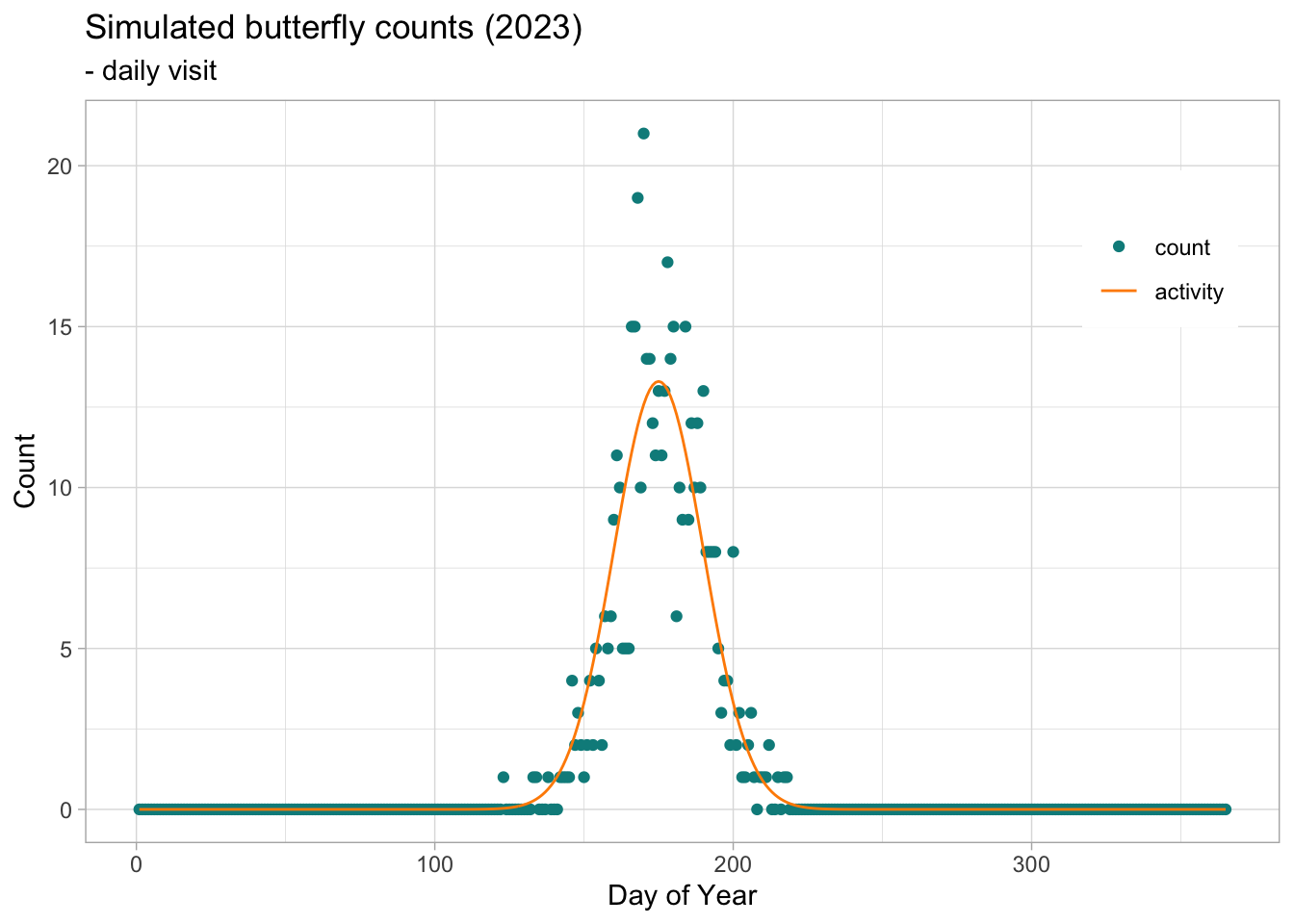
We illustrate how the timeseries_sim() function works with a simple case where we simulate butterfly counts for a univoltine species with a Gaussian pattern (i.e. one generation with a normal distribution), where the peak abundance is observed on day 175 with a standard deviation of 15 days.
The object returned by the timeseries_sim() function contains 1) a data.frame NAME$timeseries with the time series and 2) a data.frame NAME$parms with the parameters used for the simulation. The parameters are the population growth rate (growth.rate), the initial population size (init.size) measured in number of individuals expected over the season, the peak of the activity curve (act.mean) measured in days and the width of the activity curve (act.sd) measured in standard deviation.
Note
Note that not all the sampling parameters used for the simulation are included in the parms object; activity.type' (the distribution function used to define the activity curve),sample.type’ (the sampling procedure used to sample random counts along the activity curve) and `abund.type’ (the type of growth rate, deterministic or with a log-normal process error) are missing.
Simulate Data Sampling Process
With the timeseries_sim() function above we simulated a regular time series of butterfly counts, where the actual number of active butterflies of each day is drawn from a Poisson distribution with a given expectation, defined by the activity curve along a day-of-year vector \(j\), following the probability density of a normal (Gaussian) distribution with a mean equal to the peak day \(\mu\) (act.mean) and a standard deviation \(\alpha\) (act.sd). Since the integral of the probability density distribution (area under the curve) is 1, we can multiply the density by the total abundance to obtain a vector of expected abundance for each day of the year, \(\lambda_j\).
From the activity curve, we can use the rpois() function in R to draw a random value from a Poisson distribution, where \(y_i\) is the count for day \(j\) and the mean is given by the expected value \(\lambda\) on day \(j\).
\[
y_j = rpois(\lambda_j)
\]
From this simulation, we have generated the ecological process for the butterfly counts, for a given abundance distributed over a specific phenology, defined by a Gaussian curve with a peak (mean) and a breath (standard deviation).
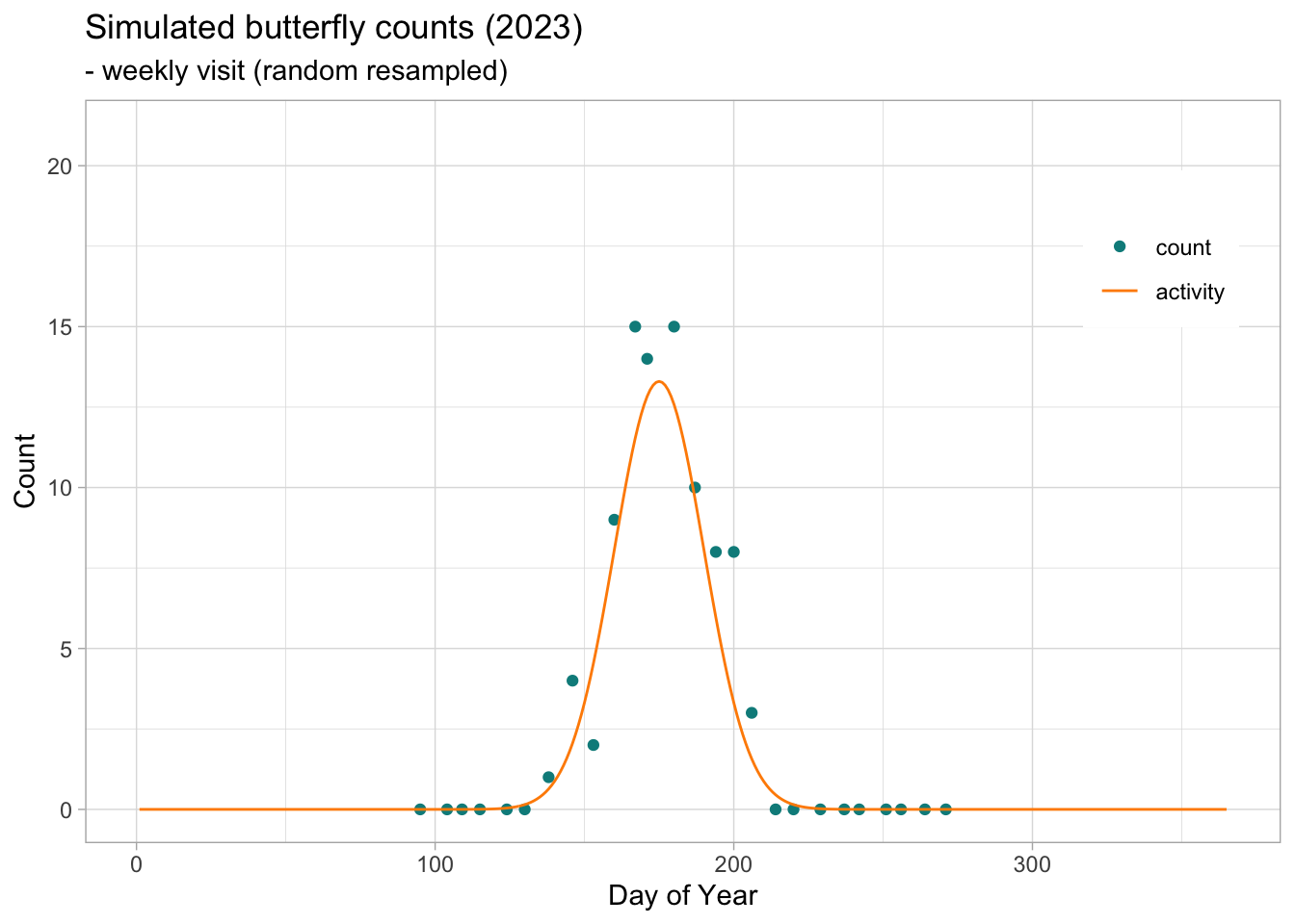
The additional structure resulting from the monitoring protocol (observation process) can now be added to the simulated time series to reproduce a specific protocol. In this first case, we will simulate a protocol with weekly visits and include some missing counts for weeks when the minimum monitoring conditions were not met or the observer was absent. To do this, we will write some new R functions. The first function will define the start and end of the monitoring season and sample one monitoring day per week throughout the season. Then we will write functions to simulate a certain level of missing weekly visits within the season. The probability of missing weeks tends to be higher at the beginning and end of the season and lower in the middle. Let’s start with the first function, which defines the monitoring season and resamples one day of the simulated time series each week. We will call the function sim2bms() as it adapts the simulated time series to the protocol of a specific Butterfly Monitoring Scheme (BMS). The function takes the time series and additional arguments to define the year we want to extract yearKeep, if the time series needs to be resampled weekly weeklySample, which day to use for the weekly resampling weekdayKeep (this can be a vector of days, e.g. c(2,3,4,5), or a specific day), and finally the monitoring season monitoringSeason, which is a vector of months, e.g. c(4,5,6,7,8,9) represents a season starting in April and ending in September. Note that this function also adds some new variables such as the date, the ISO week number and the day of the week.
Code
# data: Time series resulting from the simulation generated for 365 days# weeklySample: TRUE or FALSE; should the daily count in the time series be resampled weekly?# weekdayKeep: vector of days c(1,2,..., 7) to be sampled from for the weekly count. If the vector# contains c(2,3,4), the sampling process will be restricted to Tuesday, Wednesday or Thursday.# monitoringSeason: vector of months that define the monitoring season (e.g. April to September is c(4:9)). sim2bms <-function(data, yearKeep =NULL, weeklySample =FALSE, weekdayKeep =NULL, monitoringSeason =NULL){ btfl_ts <- data.table::data.table(data)[, site_id :=paste0("site_",sim.id)]if(!is.null(yearKeep)){ btfl_ts <- btfl_ts[years %in% yearKeep, ] } btfl_ts[ , date :=as.Date(doy, origin =paste0(years, "-01-01"))-1] btfl_ts[ , week :=isoweek(date)] btfl_ts[month(date) !=1| week <50, weekday :=rowid(week), by = .(site_id, years)]if(isTRUE(weeklySample)){if(!is.null(weekdayKeep)){ btfl_ts <- btfl_ts[weekday %in% weekdayKeep, ] } btfl_ts <- btfl_ts[btfl_ts[,.I[sample(.N, 1)], by = .(week, site_id, years)][["V1"]],] }if(!is.null(monitoringSeason)){ btfl_ts <- btfl_ts[month(date) %in% monitoringSeason, ] }return(btfl_ts) }
We can use this function to retrieve a particular year of the simulated time series and add some new variables, leaving all other parameters empty. The same function can also be used to resample weekly counts (e.g. a day from c(2:5)) and to restrict the time series to a particular monitoring season (e.g. c(4:9)).
In the example above, the activity curve represented by the line has a Gaussian shape and the counts represented by the points along the curve are independent samples from a Poisson distribution. Because we sampled a count value for 365 days (day-of-year; doy), the counts are representative of the population of active adult butterflies as if the site were visited every day. This means that a proportion of butterflies will be counted on more than one day because their lifespan is longer than one day. On Pollard transects, butterfly counts are likely to be counted and reported in this way, but at a different frequency, as visits may be weekly, fortnightly or even monthly. We can replicate this value by resampling the daily count on a weekly basis.
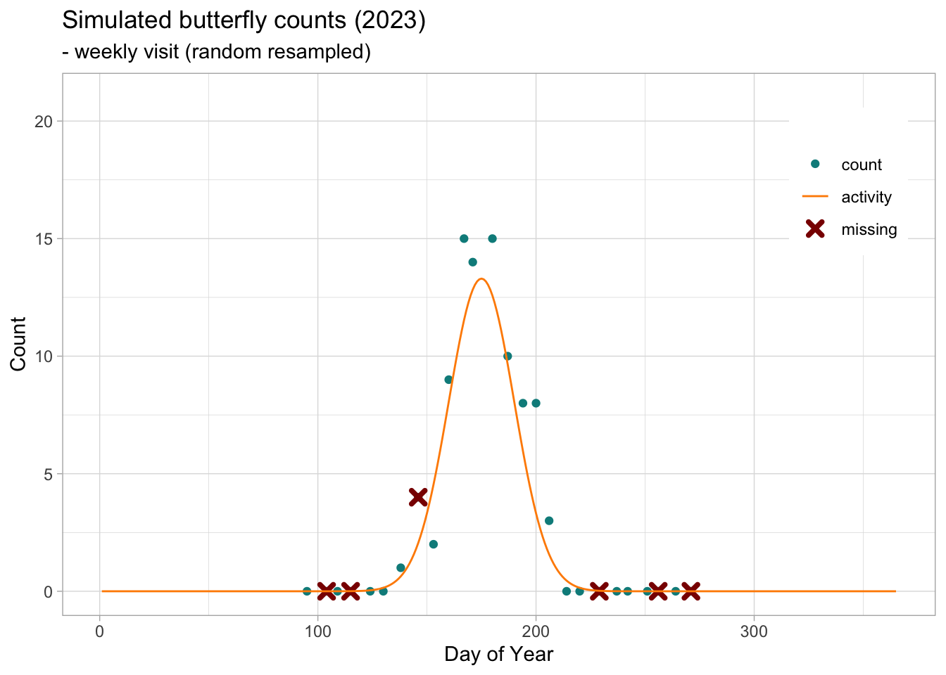
Weekly visits will not include counts outside the monitoring period, in many cases these will be ‘zeros’ as we do not expect adult butterfly activity outside the monitoring season. Some other weeks may be missing from the time series, possibly due to unsuitable weather conditions for monitoring or recorder availability. We can inform and exclude the missing visits by resampling a subset of the weekly counts.
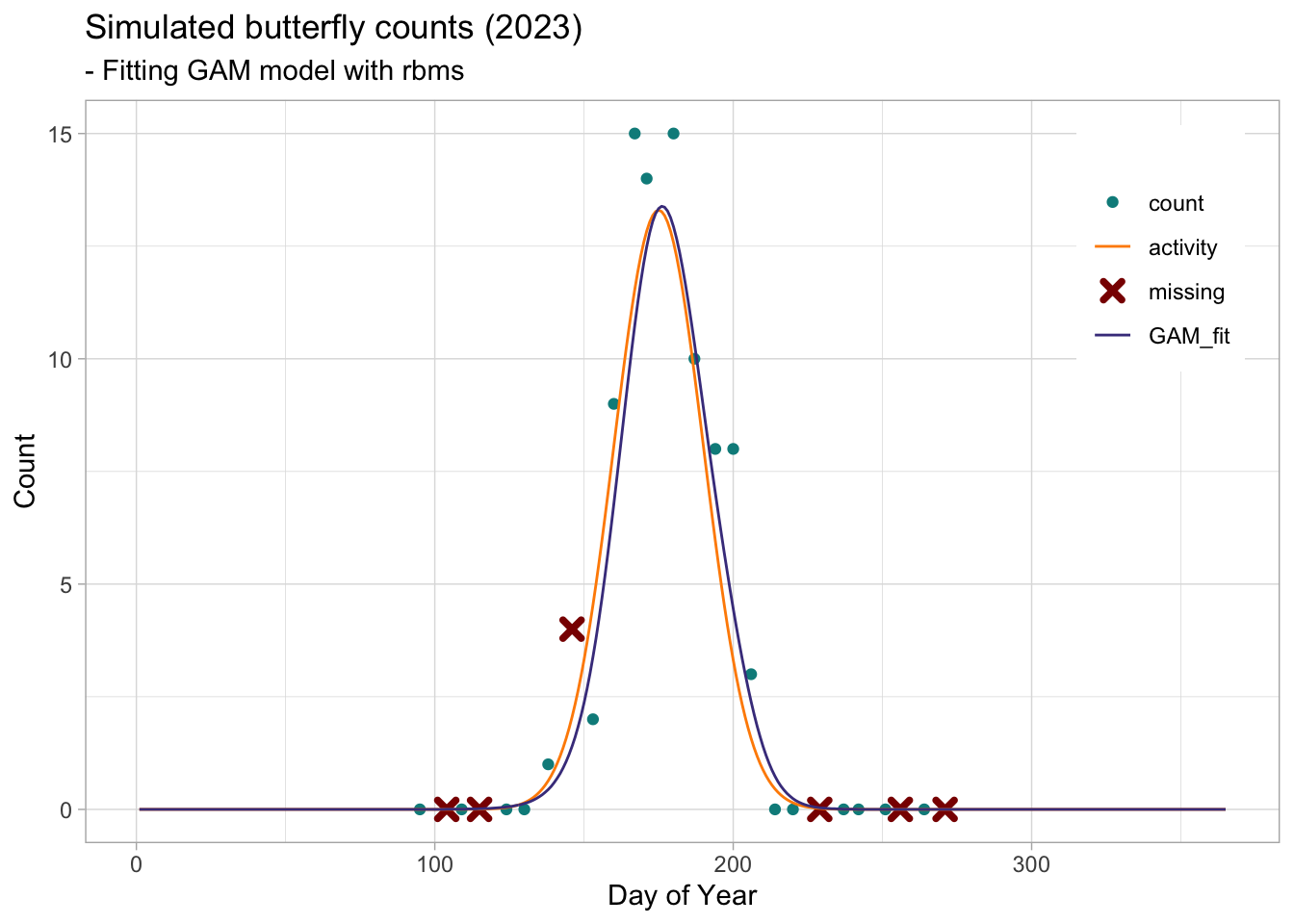
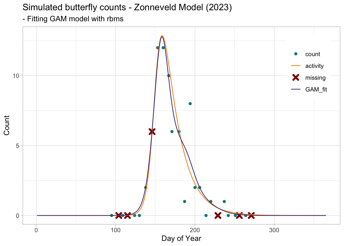
We will use the simulation to test the GAM method implemented in the R package rbms(Schmucki, Harrower A., and Dennis B. 2022). As recorders only report the number of butterflies observed, zeros are generally not reported, but can be inferred from the visit dates (e.g. we can infer zeros for the dates when monitoring took place but no individuals were reported).
The flight curve computed by the rbms::flight_curve() function is stored in the …$pheno object, where the days of the year are stored in the variable trimDAYNO and the standardised flight curve in the variable NM. The NM variable is scaled to an area under the curve (AUC) that sums to 1. To compare the flight curve derived from the GAM with the activity curve used for the simulation, we must rescale them to the same AUC, in other words we must rescale the activity curve to have an AUC of 1 or rescale the NM to the population size used for the simulation. Here we will rescale the NM to match the population size of the simulation, this will allow us to display the curves and counts on the same graph with the correct scale.
To compare the fitted curve with the activity curve, we should use a standard AUC of 1 to allow a fair comparison between models fitted to different population sizes. Using the standardised activity curve and the GAM generated flight curve (NM), we can calculate the Root Mean Squared Error (RMSE) to estimate the goodness of fit of the flight curve generated by the rbms package.
where \(y_i\) is the NM value at time \(i\) and \(\tilde{y}_i\) the value from the standardized activity curve at time \(i\), from day \(1\) to \(n\) of the monitoring season.
Non Gaussian flight curve
The same procedure can be applied to flight curves with more complex shapes. Here we generate a time series of butterfly counts from a known flight curve (adult activity) using a simulation of a Zonneveld model.
In our first scenario, we apply the method to a simple case study of a single univoltine species monitored over 15 years at 100 sites. In this case, the observed population trends follow a consistent trajectory with a known growth rate.
Edwards, Collin, Cheryl Schultz, David Sinclair, Daniel Marschalek, and Elizabeth Crone. 2023. “Estimating Butterfly Population Trends from Sparse Monitoring Data Using Generalized Additive Models.” December 8, 2023. https://doi.org/10.1101/2023.12.07.570644.
Schmucki, Reto, Colin Harrower A., and Emily Dennis B. 2022. “rbms: Computing generalised abundance indices for butterfly monitoring count data.”https://github.com/RetoSchmucki/rbms.