Trends Simulation

Content under construction

Multisite and trends

Here we will simulate butterfly count data for multiple sites (100), for a univoltine species that has a simple Gaussian flight curve (peak at day 175), where each population has an initial number of 500 individuals (total number of observations accumulated over the season) and a mean population growth rate of 20% over 10 years (2010 to 2020). We introduce some variation (standard deviation of 0.02) in the growth rate observed across the 100 sites.

For this simulation, we will use the timeseries_sim() function from the butterflyGamSims package and the sim2bms() function written above to reformat the simulated data into a format that can be used in the rbms package.

Code

set.seed(13276)

if(!require("butterflyGamSims")) devtools::install_github("cbedwards/butterflyGamSims")

trend_sim <- data.table()

for(i in 1:100){

      btfl_data <- timeseries_sim(nsims=1,
                  year = c(2010:2020),
                  doy.samples = seq(from=1, to=365, by=1),
                  abund.type = "exp",
                  activity.type = "gauss",
                  sample.type = "pois",
                  sim.parms = list(growth.rate = rnorm(1, mean = 0.2, sd=0.02),
                                    init.size = 500, 
                                    act.mean = 175,
                                    act.sd = 15)
                  )

      trend_sim <- rbind(trend_sim, 
                        sim2bms(data = btfl_data$timeseries, 
                              weeklySample = TRUE,
                              weekdayKeep = c(2:5),
                              monitoringSeason = c(4:9))[,
                              growth.rate := btfl_data$parms$growth.rate][,
                              site_id := paste0("site_id", i)])

}
knitr::kable(head(trend_sim))

Code

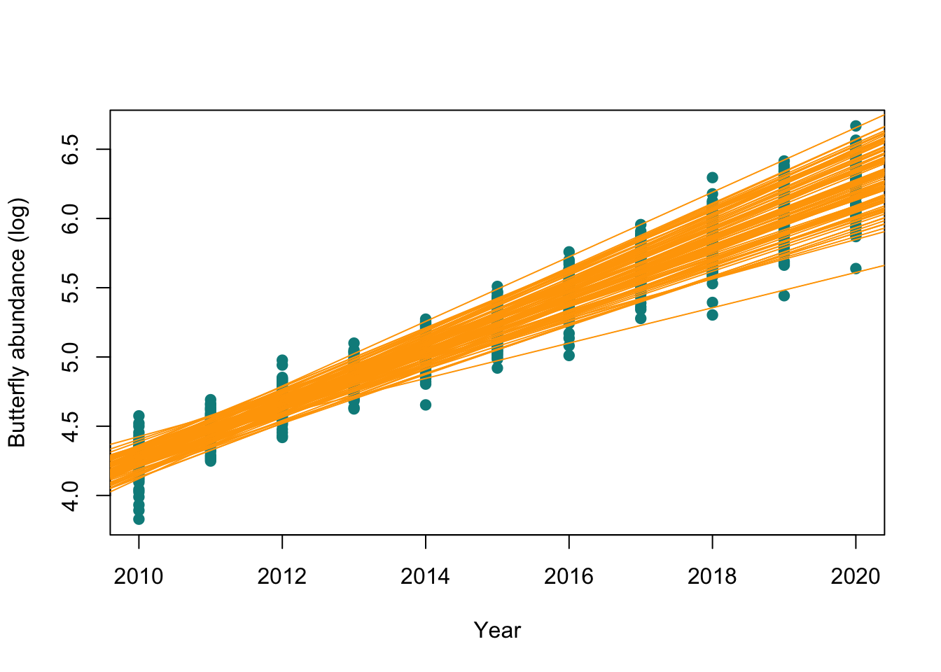
## plot and add lm

trend_sim[, y_count := sum(count), by = .(site_id, years)]
plot(unique(trend_sim[, .(years, log(y_count))]), pch = 19, col = "darkcyan", 
      ylab = "Butterfly abundance (log)", xlab = "Year")

for(i in 1:100){
    abline(lm(log(y_count) ~ years, data = trend_sim[site_id == paste0("site_id", i), .(years, y_count)]),  
            col = 'orange')
}

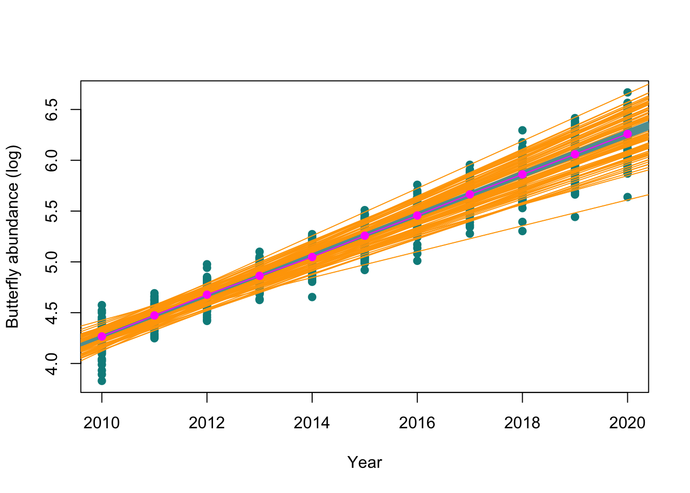
The overall trend can be calculated by fitting a Generalized Linear Model (GLM), with a Poisson error distribution on the simulated dataset. Note that here we did not include the site effect as all sites had the same abundance (500 individuals) and we excluded the intercept from our model. To illustrate the effect of the variation in the trends across sites on our overall trend estimate, we can bootstrap (resample with replacement) the sites and fit the GLM on the bootstrap sample. We can generate 100 (or more) iterations to illustrate the variation around the trend derived from our 100 sites.

Code

plot(unique(trend_sim[, .(years, log(y_count))]), pch = 19, col = "darkcyan", 
      ylab = "Butterfly abundance (log)", xlab = "Year")

for(i in 1:100){
    abline(lm(log(y_count) ~ years, data = trend_sim[site_id == paste0("site_id", i), .(years, y_count)]),  
            col = 'orange')
}

for(i in seq_len(100)){

boot_site <- sample(unique(trend_sim$site_id), trend_sim[, uniqueN(site_id)], replace = TRUE)

#points(c(2010:2020), as.numeric(coef(glm(y_count~ factor(years) - 1, data = trend_sim[site_id %in% boot_site, ],
#                                           family = "poisson"))), col = 'magenta', pch = 19)

abline(lm(as.numeric(coef(glm(y_count~ factor(years) - 1, data = trend_sim[site_id %in% boot_site, ], 
                              family = "poisson"))) ~ c(2010:2020)), col = 'cadetblue', type = 'l')
}

points(c(2010:2020), as.numeric(coef(glm(y_count~ factor(years) - 1, data = trend_sim, family = "poisson"))), 
      col = 'magenta', pch = 19)
points(c(2010:2020), as.numeric(coef(glm(y_count~ factor(years) - 1, data = trend_sim, family = "poisson"))), 
      col = 'magenta', type = 'l')